Kalman Filter in Robotics

What is Kalman Filter in Robotics?

The Kalman filter is a mathematical algorithm that combines noisy measurements with a model of how a system evolves to produce the optimal estimate of the system's true state. In robotics, it fuses GPS, IMU, encoders, and other sensors to give one clean position and velocity.

How It Works

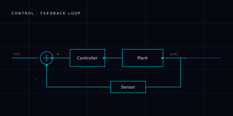
At each step the filter does two things. Predict: it uses a motion model (e.g., constant velocity) to advance its belief forward in time, growing the uncertainty. Update: when a new sensor reading arrives, it computes how much to trust the reading vs the prediction (the Kalman gain) and pulls the estimate toward the measurement. The math optimally minimises mean-squared error if the system is linear and noise is Gaussian. Implementations come in under 50 lines of Python — but tuning the process and measurement covariance matrices is its own art.

Real-World Example

Apollo 11's onboard computer used a Kalman filter to navigate to the Moon — the algorithm's first famous job. Every modern drone autopilot (PX4, ArduPilot) runs one to fuse GPS, barometer, and IMU into a single position and attitude estimate. Self-driving stacks fuse radar, camera, and IMU with Kalman-family filters. India's Mars Orbiter Mission, ESA's probes, and NASA's rovers have all leaned on Kalman filtering for trajectory estimation — it is the default tool for state estimation across the world's space and robotics programs.

The math (predict and update)

The filter tracks two things: the state estimate x (e.g. position and velocity) and its uncertainty, the covariance matrix P. Each cycle has two stages.

Predict — advance the state with the motion model F, and grow uncertainty by the process noise Q:

x = F·x + B·u
P = F·P·Fᵀ + Q

Update — when a measurement z arrives (related to the state by H, with measurement noise R), compute the Kalman gain K and correct:

y = z − H·x                 # innovation (measurement surprise)
S = H·P·Hᵀ + R              # innovation covariance
K = P·Hᵀ·S⁻¹                # Kalman gain
x = x + K·y                 # corrected state
P = (I − K·H)·P             # shrunk uncertainty

The gain K is the whole story: when the sensor is trustworthy (small R), K is large and the estimate jumps to the measurement; when the sensor is noisy, K is small and the filter leans on its prediction. It works out this trade-off optimally — minimum mean-squared error — whenever the system is linear and the noise is Gaussian.

In code (1D constant-velocity, ~15 lines)

import numpy as np
x = np.array([[0.], [0.]])          # position, velocity
P = np.eye(2) * 500.                 # start very uncertain
F = np.array([[1., dt], [0., 1.]])   # constant-velocity model
H = np.array([[1., 0.]])             # we only measure position
Q = np.array([[0.05, 0.], [0., 0.05]])
R = np.array([[2.0]])                # sensor variance

def step(z):
    global x, P
    x = F @ x                        # predict
    P = F @ P @ F.T + Q
    y = z - H @ x                    # update
    S = H @ P @ H.T + R
    K = P @ H.T @ np.linalg.inv(S)
    x = x + K @ y
    P = (np.eye(2) - K @ H) @ P
    return x

Notice the filter estimates velocity it never directly measures — it infers it from how position changes, which is the quiet magic of state estimation.

Tuning Q and R (where the real work is)

The equations are easy; making a filter behave is not. Two knobs dominate:

• R (measurement noise) — set it from the sensor's actual variance (datasheet or empirical). Too small and the filter chases every sensor glitch; too large and it ignores good data.
• Q (process noise) — how much you trust your motion model. Too small and the filter becomes over-confident and lags real changes (or diverges when the model is wrong); too large and the output stays jittery. Q is usually hand-tuned until the estimate tracks without over-reacting.

A useful diagnostic: the innovation y should look like zero-mean noise. If it trends, your model or Q is wrong.

When the plain Kalman filter isn't enough

The classic KF assumes linear dynamics and Gaussian noise. Real robots break both:

• Nonlinear models (a robot's heading, range-bearing sensors) → Extended Kalman Filter (linearize with Jacobians) or Unscented Kalman Filter (propagate sample points, more accurate for strong nonlinearity).
• Non-Gaussian / multi-modal beliefs (kidnapped-robot localization, "am I in room A or the identical room B?") → particle filter, which represents the belief with thousands of weighted samples.
• Large SLAM back-ends → factor graphs (GTSAM), which generalize the same least-squares idea across a whole trajectory.

Divergence is the classic failure: if the true state leaves the region the covariance says is plausible (bad model, unmodeled bias, wildly wrong R), the filter grows over-confident and stops trusting correct measurements. Watching the innovation and covariance is how you catch it.

Why It Matters for Robotics

If you want to do serious robotics — drones, autonomous cars, mobile robots — you must understand Kalman filtering. It's a standard topic in senior robotics interviews everywhere, and it's the gateway to modern state-estimation methods like the EKF, UKF, and factor graphs.

Try It Yourself

Open /visualizer and load the Kalman demo: play with measurement noise, process noise, and watch the filter converge. Then implement the 1D position-velocity filter above on a noisy random-walk simulation and try mistuning Q and R to see it lag or jitter.

Quick Quiz

🧠
Quick Quiz
3 questions
1.A Kalman filter combines:
A.Two cameras only
B.A motion model with noisy measurements
C.Two batteries in parallel
D.No data at all
2.The Kalman gain controls:
A.Sensor brightness
B.How much to trust the new measurement vs the prediction
C.Power consumption
D.Motor speed
3.Standard Kalman filtering assumes:
A.Nonlinear dynamics
B.Linear dynamics and Gaussian noise
C.Discrete-only states
D.Pure deterministic systems

Further Reading

• Sensor Fusion
• Extended Kalman Filter
• Particle Filter
• Imu
• Gps Module

Ask R2 About This

Open the R2 Co-pilot (press ⌘K anywhere on R2BOT) and ask: "Explain the Kalman filter to a beginner, then show me the predict/update equations for a 2D position tracker." You'll get a tailored, sourced answer in seconds.

Press ▶ Run to execute. First run downloads Python (~6MB) — only happens once per page.